



ElegantVLA: Learning When to Think for Efficient Vision-Language-Action Models
VLA가 매 control step마다 전부 “생각”하지 않고, 현재 로봇 phase가 안정적인지/민감한지를 보고 Vision-LLM과 action head 계산을 동적으로 재사용하는 plug-in inference scheduler
기존 VLA는 vision encoder, LLM, action-generation module(such as autoregressive decoder, flow model, or diffusion head)을 매 제어 주기마다 실행하기 때문에 latency가 크고 control frequency가 낮아진다. 기존 acceleration 방법론들은 token pruning, caching, layer skipping, quantization, action-head acceleration처럼 특정 모듈만 줄이거나 fixed rule을 쓰는 경우가 많아서 로봇 제어 과정의 phase별 계산 수요 차이를 충분하게 반영하지 못한다.
ElegantVLA는 로봇 manipulation에서 movement 구간은 상대적으로 안정적이고, contact·alignment·grasping·insertion·placement 같은 구간은 더 정밀한 계산이 필요하다는 점에 주목한다. ElegantVLA는 frozen VLA 위에 lightweight RL scheduler를 붙여 CKA(centered kernel alignment) 기반 representation stability, gripper speed, end-effector translation speed, end-effector rotation speed, episode progress를 보고 Vision-LLM은 5단계, action head는 3단계 계산 모드 중 하나를 선택한다. 즉 핵심은 “계산량을 고정적으로 줄이는 것이 아니라, task phase에 따라 어디서 full compute를 쓰고 어디서 cache/reuse할지 학습하겠다”이다.
결과적으로 CogACT에서 최대 3.77×, GR00T에서 최대 2.55×, 실제 Franka 실험에서 2.18× FLOPs speedup을 얻으면서 평균 task success를 유지하거나 약간 개선했다.
Introduction
큰 VLM/LLM backbone과 iterative action head를 매 control step마다 모두 실행하면, 제어 주기가 10–20Hz 수준에 묶이고 real-time manipulation에서 observation-action delay가 커진다. 모든 step이 같은 난이도를 갖는 것이 아닌데, 기존 VLA는 거의 매 step마다 같은 계산을 반복한다는 것이 이 논문의 출발점이다. 논문이 던지는 핵심 질문 및 핵심 문제는 아래와 같다:
로봇이 지금 안정적인 이동 phase에 있는가, 아니면 contact/alignment/grasp/placement처럼 정밀한 판단이 필요한 phase에 있는가? 그리고 그에 맞춰 Vision-LLM과 action head 계산량을 다르게 배분할 수 있는가?
- 명시적인 phase label 없이 per-step 계산 수요를 어떻게 추정할 것인가?
- Vision-LLM과 action head를 따로따로 줄이다가 error accumulation이 생기지 않도록 어떻게 joint scheduling할 것인가?
Preliminary: notation
논문에서는 standard VLA policy를 다음과 같이 쓴다:
\[ \mathbf{z}_t = \mathcal{L}_\phi(\mathcal{E}_\phi(\mathbf{I}_t), q), \quad \hat{\mathbf{a}}_{t:t+K-1} = \mathcal{H}_\phi(\mathbf{z}_t, \mathbf{s}_t) \]$\mathbf{I}_t$는 현재 카메라 이미지, $q$는 language instruction, $\mathbf{z}_t$는 task-conditioned representation, $\mathbf{s}_t$는 robot state, $\hat{\mathbf{a}}_{t:t+K-1}$는 action chunk, $\mathcal{E}_\phi$는 vision encoder, $\mathcal{L}_\phi$는 LLM/Vision-Language backbone, $\mathcal{H}_\phi$는 action head이다. ElegantVLA는 이 base model을 retrain하지 않고 frozen 상태로 둔 뒤, inference execution path만 바꾼다.
VLA 계산 수요는 phase마다 다르다
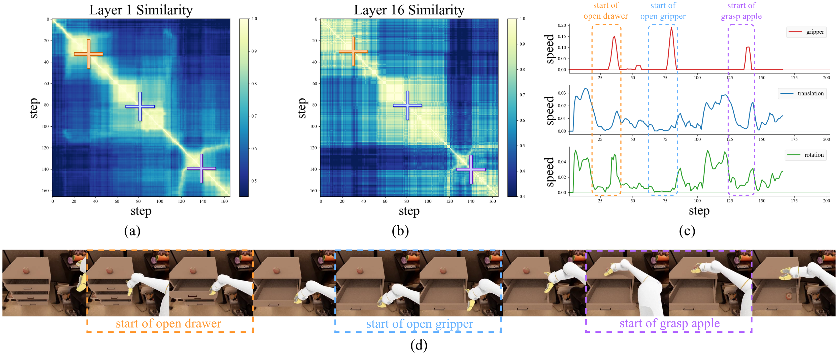 Observation motivating phase-adaptive cache scheduling
위 figure는 이 논문 전체를 이해하는 key figure이다. Drawer opening과 apple grasping rollout에서 다음을 보여준다:
- LLM first layer representation의 pairwise CKA similarity
- LLM final layer representation의 pairwise CKA similarity
- gripper, translation, rotation speed
- 실제 robot rollout
위 figure를 보면 모든 control step이 균일하게 어렵지 않다는 것을 알 수 있다. 안정적인 구간에서는 representation similarity가 높고, phase transition이나 goal-sensitive stage에서는 representation 변화가 커지는 것을 확인할 수 있다. 또한 final-layer representation 변화가 first-layer representation에서도 어느 정도 관찰된다는 것 또한 확인할 수 있다. 따라서 논문의 저자들은 비싼 full LLM inference를 다 실행하지 않고도, first LLM layer의 CKA similarity를 lightweight probe로 사용해 cache/recompute 결정을 내릴 수 있다고 주장한다.
논문에서는 최근 full computation 시점의 anchor hidden-state matrix를 $\mathbf{H}_{\tau}$, 현재 first-layer hidden-state matrix를 $\mathbf{H}_t$라고 두고, $\rho_{t} = \text{CKA}(\mathbf{H}_{t}, \mathbf{H}_{\tau})$를 계산한다. 이 값이 클수록 현재 visual-language representation이 cache와 비슷하므로 reuse가 안전하다고 판단할 수 있다.
Method
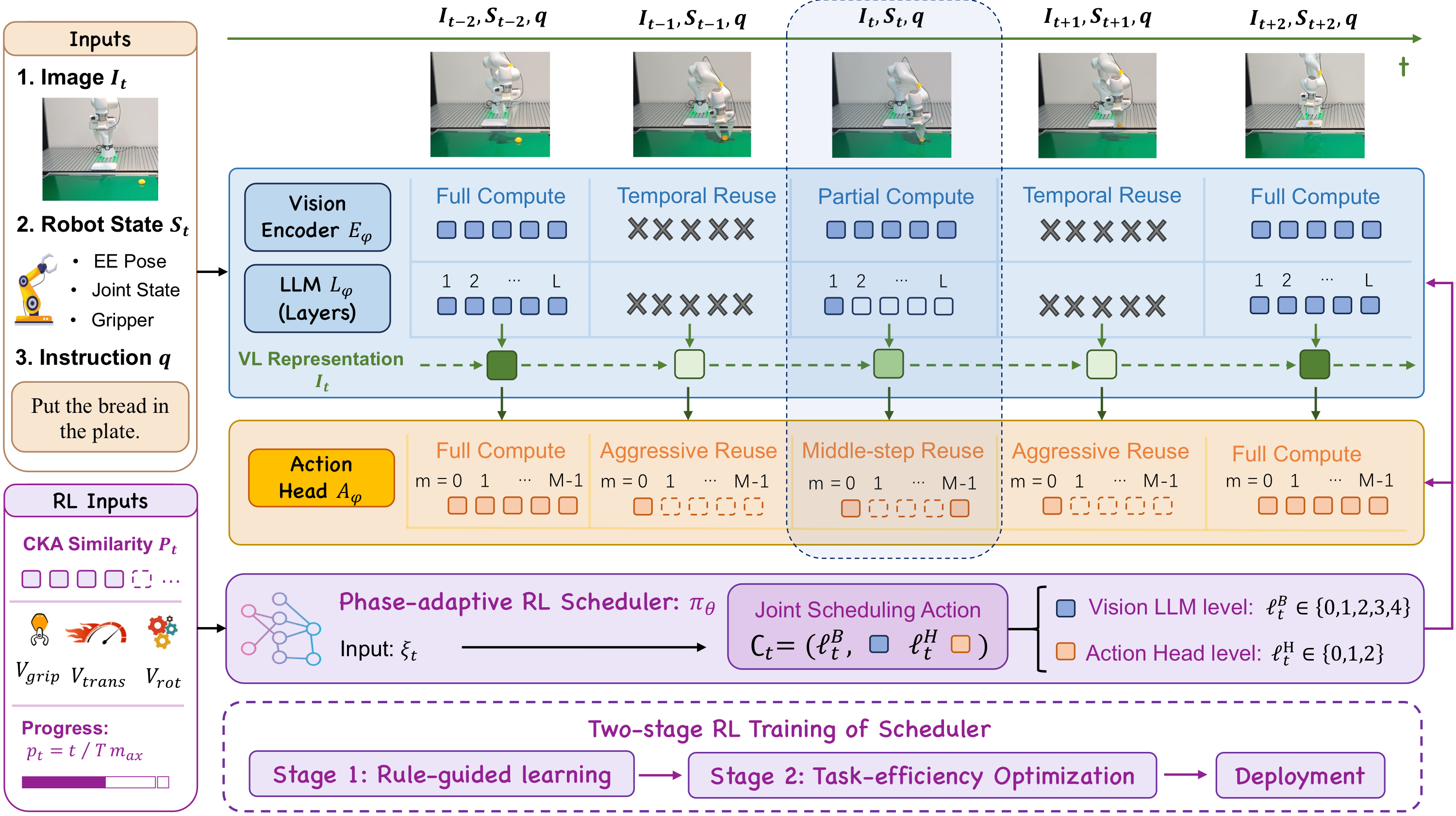 Framework Overview
ElegantVLA는 base VLA를 바꾸지 않고 이미 학습된 VLA의 inference path를 scheduler가 step마다 선택한다. 논문에서는 scheduler action을 다음처럼 정의한다:
\[ c_t = (\ell_t^B, \ell_t^H) \sim \pi_\theta(\cdot \mid \boldsymbol{\xi}_t) \]- $\ell_t^B$: Vision-LLM backbone compute level
- $\ell_t^H$: action head refinement compute level
- $\boldsymbol{\xi}_t$: scheduler observation
scheduler observation은 다음과 같다:
\[ \boldsymbol{\xi}_t = [ \rho_t, v_t^{grip}, v_t^{trans}, v_t^{rot}, p_t ]^\top \]| 입력 | 의미 | 직관 |
|---|---|---|
| $\rho_t$ | CKA-based temporal representation similarity | semantic context가 안정적인가? |
| $v_t^{grip}$ | gripper speed | gripper가 열고 닫히는 중요한 순간인가? |
| $v_t^{trans}$ | end-effector translation speed | 이동이 안정적인가, 급격한 correction이 있는가? |
| $v_t^{rot}$ | end-effector rotation speed | 자세 정렬이 민감한가? |
| $p_t = t/T_{\max}$ | normalized episode progress | episode 초반/중반/후반 중 어디인가? |
Scheduler는 Vision-LLM backbone과 action head를 함께 제어한다. Stable phase에서는 cached computation을 재사용하고, phase-sensitive moment에서는 full recomputation을 수행한다.
Vision-LLM scheduling: 5-level compute ladder
Vision-LLM backbone은 매 step image를 encoding하고 LLM layer 전체를 실행해야 하기 때문에 per-step inference cost의 큰 부분을 차지한다. ElegantVLA는 이를 5단계 compute level로 나눈다:
$\ell_t^B = 0$: Full recomputation
이 모드는 vision encoder와 LLM 전체를 모두 실행한다:
\[ \mathbf{z}_t = \mathcal{L}_\phi(\mathcal{E}_\phi(\mathbf{I}_t), q) \]이때 cache anchor와 output representation도 새로 갱신해야 한다. 사용해야 하는 상황은 다음과 같다:
- scene이 크게 바뀐 경우
- object contact가 발생하는 경우
- drawer state, object pose, spatial relation이 바뀌는 경우
- grasp, insertion, placement처럼 precision-sensitive한 경우
$\ell_t^B = 1$: Partial recomputation
이 모드에서는 vision encoder를 새로 실행하고, LLM의 first layer와 last layer만 recompute한다. 중간 LLM representation은 가장 최근 full computation에서 가져온 cache를 재사용한다:
\[ \mathbf{z}_t = \mathcal{L}_{\phi}^{\text{last}}( \bar{\mathbf{u}} , \mathcal{L}_{\phi}^{\text{first}}(\mathcal{E}_\phi(\mathbf{I}_t), q) ) \]$\bar{\mathbf{u}}$는 cached intermediate LLM states이다. 위와 같은 computation의 배경이 되는 직관은 아래와 같다:
- first layer는 현재 input image와 instruction을 반영한다.
- middle layer들은 계산량이 크고, stable phase에서는 이전 representation과 크게 다르지 않을 수 있다.
- last layer는 최종 output alignment를 위해 다시 계산해야 한다.
즉, 현재 observation sensitivity는 어느 정도 유지하면서도 비싼 intermediate Transformer block들을 줄이는 방식이다.
$\ell_t^B \in {2, 3, 4}$: Temporal reuse
나머지 경우는 vision encoder와 LLM을 모두 skip하고, 가장 최근 visual-language representation $\bar{\mathbf{z}}$를 그대로 사용한다. $\ell_{t}^{B} = j$일 때, $j - 1$ consecutive control steps 동안 reuse한다.
| Vision-LLM level | 실행 방식 | reuse 정도 |
|---|---|---|
| $\ell^B=0$ | vision encoder + full LLM | 없음 |
| $\ell^B=1$ | vision encoder + first/last LLM, middle cached | 중간 |
| $\ell^B=2$ | cached VL representation reuse | 약한 temporal reuse |
| $\ell^B=3$ | cached VL representation reuse | 더 긴 temporal reuse |
| $\ell^B=4$ | cached VL representation reuse | 가장 aggressive reuse |
Action-head scheduling: 3-level denoising/refinement reuse
Vision-LLM이 high-level semantic reasoning을 담당한다면, action head는 low-level continuous action generation을 담당한다. 특히 diffusion/flow/action refinement 계열 action head는 여러 refinement step을 반복하기 때문에, 여기에도 큰 temporal redundancy가 있다.
논문은 iterative action head를 다음처럼 쓴다:
\[ \mathbf{x}_{t}^{m + 1} = \mathcal{F}_{\phi}^{m}(\mathbf{x}_{t}^{m}, \mathbf{z}_{t}, \mathbf{s}_{t}), \quad m = 0, \dots, M - 1 \]$\mathbf{x}_{t}^m$은 $m$-번째 refinement step의 intermediate action state이다. ElegantVLA는 action head에 대해 3단계 compute level을 둔다.
$\ell_t^H = 0$: Full refinement
이 모드에서는 모든 refinement step을 새로 계산한다.
\[ \mathcal{R}(\ell_t^H)=\varnothing \]$\mathcal{R}(\ell_t^H)$는 cache에서 재사용되는 refinement step들의 set이다. 다음과 같은 상황들에서 적합하다:
- contact 직전/직후
- grasp pose가 민감한 경우
- placement/release가 중요한 경우
- robot state가 급격히 변하는 경우
$\ell_t^H = 1$: Middle-step reuse
이 모드에서는 middle refinement update만 cache에서 재사용하고, boundary step은 recompute한다:
\[ \mathcal{R}(\ell_t^H)=\{1,\ldots,M-2\} \]직관적으로는 다음과 같다:
- 처음 step은 현재 $\mathbf{z}_t$, $\mathbf{s}_t$를 반영하기 위해 새로 계산한다.
- 중간 denoising/refinement 방향을 이전 step과 비슷하다고 보고 reuse한다.
- 마지막 step은 output adaptation을 위해 다시 계산한다.
따라서 full recompute보다는 싸지만, output precision을 어느정도 유지한다.
$\ell_t^H = 2$: Aggressive reuse after first refinement
\[ \mathcal{R}(\ell_t^H)=\{1,\ldots,M-1\} \]첫 refinement만 새로 계산하고, 이후 update는 cache된 $\bar{\mathbf{\Delta}}^{m}$을 사용한다. 재사용되는 step에서는 다음과 같이 update한다:
\[ \mathbf{x}^{m+1}_{t} = \mathbf{x}^{m}_{t} + \bar{\mathbf{\Delta}}^{m} \]즉, 이전 실행에서 얻은 refinement direction/update를 현재 step에 적용한다. stable motion에서는 action-generation trajectory가 크게 변하지 않기 때문에 이런 reuse가 가능하다. 하지만 contact나 fine alignment에서는 위험할 수 있으므로 scheduler가 $\ell_{t}^{H} = 0$ 또는 $\ell_{t}^{H} = 1$을 선택해야 한다.
Joint Scheduling
ElegantVLA는 semantic redundancy와 control redundancy를 분리해서 본다:
- Vision-LLM redundancy는 주로 이미지, instruction, scene semantics가 안정적인지와 관련된다.
- Action-head redundancy는 robot motion이 smooth한지, refinement trajectory가 안정적인지와 관련된다.
둘은 관련 있지만 완전하게 같지는 않다. 예를 들어:
scene semantics는 안정적이지만 action은 정밀해야 하는 경우
- 물체가 계속 같은 위치에 보이더라도, grasp 직전에는 action head를 full recompute해야 할 수 있다.
Vision-LLM은 새로 계산해야 하지만 action refinement는 reuse 가능한 경우
- high-level visual-language representation은 refresh해야 하지만, motion trajectory 자체는 smooth할 수 있다.
둘 다 reuse 가능한 경우
- 단순 transport phase에서는 semantic context도 안정적이고 action trajectory도 smooth하다.
둘 다 full recompute해야 하는 경우
- 접촉, 삽입, drawer opening/closing, placement, moving target correction 같은 구간이다.
그래서 ElegantVLA는 $\ell_{t}^{B}$와 $\ell_{t}^{H}$를 하나의 joint action으로 선택한다. 가능한 조합은 기본적으로 $5 \times 3 = 15$개이다.
RL scheduler: rule-guided pretraining + task-efficiency optimization
Base VLA는 frozen인 상태로 scheduler는 Maskable PPO로 학습한다. Action masking이 필요한 이유는 Vision-LLM에서 multi-step reuse를 선택하면, 그 reuse window 안에서는 backbone choice가 고정되기 때문이다. 반면 action head는 여전히 매 control step마다 decision이 필요하다.
Stage 1: Rule-guided learning
한 episode에는 수백 개 scheduling decision이 있지만, 성공/실패 feedback은 episode 끝에야 나오기 때문에 처음부터 sparse terminal success와 FLOPs만 보고 RL을 학습시키기에는 어렵다. 따라서 Stage 1에서는 rule-guided teacher를 사용해 dense shaping reward를 준다:
\[ r_t^{(1)} = r_t^{succ} - \lambda_C r_t^{FLOPs} - \lambda_B d(\ell_t^B, \tilde{\ell}_t^B) - \lambda_H d(\ell_t^H, \tilde{\ell}_t^H) - \lambda_R k(\ell_t^B) \]| 항목 | 의미 |
|---|---|
| $r_t^{succ}$ | task success 관련 reward |
| $r_t^{FLOPs}$ | 선택한 execution path의 computation cost |
| $\tilde{\ell}_t^B, \tilde{\ell}_t^H$ | rule-guided teacher가 제안하는 compute level |
| $d(\cdot,\cdot)$ | teacher decision과 scheduler decision의 차이에 대한 penalty |
| $k(\ell_t^B)$ | Vision-LLM temporal reuse horizon |
| $\lambda_C,\lambda_B,\lambda_H,\lambda_R$ | 각 penalty의 weight |
이 단계의 목적은 destructive exploration을 막고, scheduler가 대략적으로 “안정적인 구간에서는 reuse, 민감한 구간에서는 recompute”하는 policy를 배우게 하는 것이다.
Stage 2: Task-efficiency optimization
Stage 2에서는 teacher shaping term을 제거하고 task-efficiency feedback을 직접 최적화한다. 즉, hand-designed rule을 그대로 따르는 것이 아니라, 실제 task success와 compute saving 사이의 trade-off를 RL이 조정하게 한다. 논문에서는 ElegantVLA의 성능은 단순히 더 aggressive reuse해서 나온 것이 아니라, 어느 순간에 reuse를 풀어야 하는지 학습했기 때문에 나온다고 주장한다.
Experiments
논문은 ElegantVLA를 크게 세 가지 관점에서 평가한다:
- simulation에서 task success와 FLOPs speedup이 동시에 개선되는가?
- FLOPs 감소가 실제 latency 감소와 control frequency 증가로 이어지는가?
- Vision-LLM scheduling, action-head scheduling, two-stage RL scheduler가 각각 실제로 필요한가?
실험은 주로 SimplerEnv에서 CogACT와 GR00T를 대상으로 수행하고, 추가로 Franka Research 3 기반 real-world manipulation task에서 검증한다. 중요한 점은 base VLA인 CogACT와 GR00T는 frozen 상태로 유지하고, ElegantVLA는 inference execution path만 바꾼다는 것이다.
Simulation setup
Simulation에서는 SimplerEnv benchmark를 사용한다. CogACT 실험은 Google Robot 계열 task를 Visual Matching과 Variant Aggregation setting으로 나누어 평가한다. GR00T 실험은 Google Robot suite와 WidowX suite에서 평가한다.
CogACT task group은 다음과 같다:
| Task group | 의미 |
|---|---|
| PickCan | Coke can을 grasp하는 task |
| MoveNear | target object를 reference object 근처로 이동시키는 spatial relation task |
| Drawer | top/middle/bottom drawer opening/closing을 포함하는 drawer manipulation task |
| PutDrawer | object를 drawer 안에 넣는 task |
GR00T에서는 Google Robot 6개 task와 WidowX 7개 task를 사용한다.
| Robot suite | Tasks |
|---|---|
| Google Robot | Close Drawer, Move Near, Open Drawer, Pick Coke Can, Pick Object, Place in Closed Drawer |
| WidowX | Carrot on Plate, Close Drawer, Open Drawer, Eggplant in Basket, Eggplant in Sink, Spoon on Towel, Stack Cube |
각 결과는 기본적으로 success rate / FLOPs speedup 형태로 보고된다. Speedup은 full-computation baseline을 1.00×로 둔 상대값이다.
Main result 1: CogACT on SimplerEnv
CogACT 결과에서는 ElegantVLA가 기존 acceleration baseline보다 훨씬 큰 speedup을 얻으면서 평균 success도 가장 높게 나온다.
| Setting | Full CogACT | ElegantVLA | 핵심 해석 |
|---|---|---|---|
| Visual Matching | 74.80% / 1.00× | 77.59% / 3.72× | 성공률을 약간 개선하면서 약 3.7배 FLOPs speedup |
| Variant Aggregation | 61.30% / 1.00× | 72.54% / 3.77× | generalization setting에서 성공률 개선폭이 더 큼 |
Visual Matching에서는 full CogACT의 평균 success가 74.80%인데, ElegantVLA는 77.59%를 얻으면서 3.72× speedup을 달성한다. Variant Aggregation에서는 full CogACT가 61.30%인데, ElegantVLA는 72.54%까지 올라가고 3.77× speedup을 얻는다.
특히 Drawer 계열 task에서 성능 향상이 두드러진다. 이는 drawer opening/closing처럼 contact와 state transition이 중요한 task에서 scheduler가 모든 step을 동일하게 줄이는 것이 아니라, 중요한 phase에서는 recomputation을 유지하고 안정적인 phase에서는 reuse를 사용하는 방식이 효과적이라는 것을 보여준다.
Main result 2: GR00T on SimplerEnv
GR00T에서도 비슷한 경향이 나타난다. ElegantVLA는 Google Robot suite에서는 평균 success를 개선하고, WidowX suite에서는 평균 success를 거의 유지하면서 2.5× 수준의 speedup을 얻는다.
| Suite | Full GR00T | ElegantVLA | 핵심 해석 |
|---|---|---|---|
| Google Robot | 71.08% / 1.00× | 75.00% / 2.35× | 성공률과 speedup 모두 개선 |
| WidowX | 57.93% / 1.00× | 58.07% / 2.55× | 성공률은 거의 유지하면서 큰 speedup |
| Overall success | 64.00% | 65.88% | speedup은 suite별로 2.35×, 2.55× |
다만 모든 task에서 성공률이 오르는 것은 아니다. 일부 pickup/placement task에서는 baseline보다 약간 낮은 success가 나오기도 한다. 따라서 이 논문의 핵심 claim은 “항상 성공률을 올린다”가 아니라, 평균 task success를 유지하거나 약간 개선하면서 inference compute를 크게 줄인다에 가깝다.
Real-world experiment: Franka Research 3
Real-world 실험은 Franka Research 3에서 수행한다. Hardware setup은 Franka Research 3 robot, Intel RealSense D435i cameras, Polymetis controller, RTX 4090 기반 GR00T policy server로 구성된다. 카메라는 front-mounted eye-to-hand camera와 wrist-mounted eye-in-hand camera를 함께 사용한다. 각 task는 10 trials씩 평가한다.
Real-world task는 총 6개이다.
| Task | Full GR00T | ElegantVLA |
|---|---|---|
| Phone Stand | 60.00% / 1.00× | 60.00% / 2.18× |
| Pen Holder | 70.00% / 1.00× | 70.00% / 2.24× |
| Stack Bowls | 40.00% / 1.00× | 40.00% / 2.01× |
| Pineapple Bun | 70.00% / 1.00× | 80.00% / 2.31× |
| Toast | 70.00% / 1.00× | 80.00% / 2.21× |
| Chocolate | 60.00% / 1.00× | 60.00% / 2.11× |
| Average | 61.67% / 1.00× | 65.00% / 2.18× |
Phone Stand, Pen Holder, Stack Bowls는 stationary precision task이고, Pineapple Bun, Toast, Chocolate은 conveyor-belt 위의 moving target을 집어서 plate로 옮기는 task이다. ElegantVLA는 stationary task에서는 success를 유지하고, moving-target task인 Pineapple Bun과 Toast에서는 success를 70%에서 80%로 개선한다.
이 결과는 latency-sensitive한 task에서 inference acceleration이 단순한 FLOPs 절감 이상의 의미를 가질 수 있음을 보여준다. Moving target task에서는 observation-action delay가 크면 robot이 과거 위치를 기준으로 움직이게 되는데, ElegantVLA는 per-step latency를 줄여 더 빠른 closed-loop correction을 가능하게 한다.
Latency and control frequency
논문은 FLOPs speedup뿐만 아니라 실제 latency와 control frequency도 측정한다. GR00T SimplerEnv에서 RTX 4090 기준 결과는 다음과 같다.
| Suite | Full GR00T | ElegantVLA |
|---|---|---|
| Google Robot | 16.64 Hz / 60.09 ms | 35.03 Hz / 28.55 ms |
| WidowX | 16.69 Hz / 59.92 ms | 37.70 Hz / 26.53 ms |
이는 control frequency로 보면 약 13.8 Hz에서 26.3 Hz로 증가한 것과 같다. 즉, ElegantVLA는 simulation profiling에서 control frequency를 2배 이상 높이고, per-step latency를 절반 이하로 줄인다. 이는 VLA acceleration에서 중요한 점이다. 단순히 FLOPs만 줄이는 것이 아니라, 실제 control loop에서 더 높은 frequency로 policy를 실행할 수 있어야 robot manipulation에 도움이 된다.
Real-world에서도 비슷한 경향이 나온다. Appendix 결과에 따르면 average per-step wall-clock latency는 72.44 ms에서 38.00 ms로 줄어든다. 이때 wall-clock speedup은 1.91×이고, FLOPs speedup은 2.18×이다.
| Metric | Full GR00T | ElegantVLA | Improvement |
|---|---|---|---|
| Real-world latency | 72.44 ms | 38.00 ms | 47.5% reduction |
| Wall-clock speedup | 1.00× | 1.91× | 1.91× |
| FLOPs speedup | 1.00× | 2.18× | 2.18× |
여기서 중요한 점은 FLOPs speedup과 wall-clock speedup이 완전히 같지는 않다는 것이다. 실제 robot system에서는 model compute 외에도 camera I/O, robot communication, framework overhead, synchronization overhead가 있기 때문이다. 따라서 robotics inference system에서는 FLOPs뿐 아니라 end-to-end latency를 함께 봐야 한다.
Ablation 1: two-stage RL scheduler가 필요한가?
논문은 Stage 1 rule-guided learning과 Stage 2 task-efficiency optimization을 비교한다.
| Setting | Stage 1 | Stage 2 |
|---|---|---|
| Visual Matching | 70.45% / 3.42× | 77.59% / 3.72× |
| Variant Aggregation | 69.03% / 3.31× | 72.54% / 3.77× |
Stage 1만 사용해도 상당한 speedup은 얻을 수 있지만, 최종 Stage 2를 적용하면 success와 speedup이 모두 개선된다. 이는 hand-designed rule을 그대로 따르는 것만으로는 충분하지 않고, 실제 task feedback을 통해 reuse/recompute trade-off를 조정해야 한다는 것을 보여준다.
즉 ElegantVLA의 성능은 단순히 더 aggressive하게 cache를 재사용해서 나온 것이 아니다. 중요한 것은 언제 reuse를 멈추고 full recomputation으로 돌아갈지 학습했다는 점이다.
Ablation 2: Vision-LLM과 action head를 함께 scheduling해야 하는가?
논문은 GR00T Google Robot task에서 Vision-LLM만 scheduling하거나 action head만 scheduling하는 경우를 비교한다.
| Method | Average success / speedup |
|---|---|
| Full GR00T | 71.08% / 1.00× |
| Force LLM Full | 68.17% / 1.46× |
| Force AH Full | 72.75% / 1.56× |
| ElegantVLA | 75.00% / 2.35× |
Force LLM Full은 Vision-LLM backbone을 항상 full computation으로 두고 action head 쪽만 줄이는 설정에 가깝다. Force AH Full은 action head를 항상 full computation으로 두고 Vision-LLM 쪽만 줄이는 설정에 가깝다. 두 경우 모두 full ElegantVLA보다 speedup이 낮다.
이 결과는 Vision-LLM과 action head가 서로 다른 종류의 temporal redundancy를 가진다는 것을 보여준다. Vision-LLM은 semantic context의 안정성과 관련되고, action head는 low-level motion continuity와 관련된다. 따라서 둘을 따로 최적화하는 것보다, 하나의 scheduler가 두 branch를 joint scheduling하는 것이 더 좋은 trade-off를 만든다.
Ablation 3: CKA와 robot speed signal이 모두 필요한가?
논문은 scheduler input도 ablation한다. 핵심 비교는 다음과 같다.
| Scheduler input | 의미 | 한계 |
|---|---|---|
| CKA + progress | semantic representation stability를 봄 | robot motion/contact complexity를 직접 보기 어려움 |
| speed + progress | gripper/EE motion continuity를 봄 | object state나 scene semantics 변화를 직접 보기 어려움 |
| CKA + speed + progress | semantic stability와 motion stability를 함께 봄 | 최종 ElegantVLA 설정 |
CKA만 있으면 Vision-LLM representation이 안정적인지는 볼 수 있지만, robot이 contact phase에 들어갔는지 또는 low-level action refinement가 필요한지는 알기 어렵다. 반대로 speed signal만 있으면 robot motion의 급격한 변화는 볼 수 있지만, drawer state 변화나 object displacement 같은 high-level semantic change를 직접 포착하기 어렵다.
따라서 CKA는 backbone reuse가 안전한지 판단하는 데 중요하고, speed signal은 action-head reuse가 안전한지 판단하는 데 중요하다. 둘을 함께 사용하는 것이 ElegantVLA의 scheduler design에서 핵심이다.
Qualitative results
논문은 real-world와 simulation rollout visualization도 제공한다. Real-world pineapple-bun pickup에서는 ElegantVLA가 full GR00T와 비슷한 pick-and-place phase를 유지하면서 2.31× 빠르게 task를 완료한다. Simulation에서도 Google Robot drawer opening과 WidowX carrot placement에서 key manipulation phase를 유지하면서 rollout을 더 빠르게 끝낸다.
Qualitative result의 핵심은 ElegantVLA가 단순히 action을 skip하거나 frame을 대충 건너뛰는 것이 아니라는 점이다. Approach, grasp/contact, placement 같은 precision-sensitive phase는 유지하고, stable motion 구간에서 redundant inference를 줄이는 방식으로 동작한다.
Experiment takeaway
실험 결과를 종합하면 ElegantVLA의 핵심 메시지는 다음과 같다.
VLA inference는 모든 control step에서 같은 양의 계산을 쓸 필요가 없다. Stable motion phase에서는 Vision-LLM과 action head의 이전 계산을 재사용하고, contact·alignment·placement처럼 민감한 phase에서는 full recomputation을 수행하면, task success를 유지하면서 latency와 FLOPs를 크게 줄일 수 있다.
특히 이 논문에서 중요한 점은 FLOPs reduction이 실제 control frequency 증가로 이어졌다는 것이다. GR00T simulation에서는 약 16–17 Hz 수준의 full-computation policy가 ElegantVLA를 통해 35–38 Hz 수준으로 올라가고, real-world에서도 평균 latency가 72.44 ms에서 38.00 ms로 감소한다. 이는 ElegantVLA가 단순한 model compression 기법이라기보다, real-time robot control을 위한 inference-time scheduling framework에 가깝다는 것을 보여준다.
Limitations
1. CKA probe도 공짜는 아니다
논문은 first-layer CKA가 lightweight probe라고 주장하지만, 실제 구현에서는 현재 first-layer hidden state를 얻기 위한 일부 forward 비용이 필요하다. 특히 aggressive reuse window 안에서 CKA를 어떻게 자주 계산하는지, 그 overhead가 전체 latency에 얼마나 반영되는지는 implementation detail이 중요하다.
2. hidden state와 action-head intermediate update에 접근 가능해야 한다
black-box VLA API처럼 내부 LLM layer state나 action denoising update에 접근할 수 없는 환경에서는 적용하기 어렵다. 이 방법은 system-level integration 권한이 있는 deployment setting에 더 적합하다.
3. real-world 실험 규모는 작다
real-world는 6 tasks × 10 trials이다. 다양한 robot morphology, camera setup, safety-critical task, cluttered environment에서의 일반화는 추가 검증이 필요하다. 논문도 real-world use에는 base policy와 동일한 validation, safety check, fallback execution이 필요하다고 명시한다.
4. FLOPs speedup과 wall-clock speedup은 다르다
real-world appendix에서 FLOPs speedup은 2.18×이지만 wall-clock speedup은 1.91×이다. 이는 실제 로봇 inference stack에서는 model compute 외에도 I/O, framework, synchronization, robot communication overhead가 존재하기 때문이다. performance engineering 관점에서는 FLOPs보다 end-to-end latency를 반드시 봐야 한다.
Personal Idea
SANTS와 매우 비슷한 문제의식을 공유한다(심지어 arXiv에 하루 간격으로 올라왔다). SANTS가 World Action Model에서 미래 video denoising을 언제 멈추고 얼마나 건너뛸지 결정하는 scheduler라면, ElegantVLA는 실제 VLA inference pipeline 안에서 Vision-LLM과 action head를 언제 full compute하고 언제 reuse할지 결정하는 scheduler이다.
둘 다 핵심은 “매 step 동일한 compute를 쓰지 말고, 현재 robot state와 task phase에 따라 inference compute를 adaptive하게 배분하자”는 것이다. 이 방향은 앞으로 VLA/WAM 계열 real-time inference에서 꽤 중요해질 것 같다. 특히 robotics에서는 평균 FLOPs보다 observation-action delay와 closed-loop control frequency가 더 직접적으로 task success에 영향을 줄 수 있기 때문에, 이런 phase-adaptive scheduler는 algorithm과 system optimization 사이의 중요한 접점이 될 수 있다.